an intuitive intro to reinforcement learning
2023-05-12
Let's look at the parts of an RL system.
We have an agent who is inside an environment.
This environment gives us a state - a snapshot of it at the current point (the step, in most cases point in time.
The agent has a policy, which based on the state, takes an action from the ones the environment offers at this point.
This makes the environment update, and returns a new state.
It also returns a reward (which can also positive, negative or zero).
By placing rewards we incentivize the agent to do something - like a mouse receiving a piece of cheese for solving a puzzle.
What exactly does it mean to have policy which takes an action?
As an example let's take what we call policy-learning, you can imagine it as a function taking in the state and outputting which action it thinks the agent should take.
This can be either deterministic (meaning it just returns the index of the action it wants to take) or most of the time it is stochastic (meaning it returns the probability of each action being the ideal).
If you have an ML-background, you can imagine this function as a simple NeuralNet with a softmax output layer.
Or just imagine it as a table holding each possible state and then the optimal action for each of them.
It's called policy-learning, because when we do training we train the policy itself.
(I won't be goin into more detail on policy-learning here,, check it out yourself)
What we can also do instead is called value-learning.
This means, instead of predicting an action, we predict the value of a future state.
Value basically means, what reward do we expect if we go into that state.
So not simply the reward we will get from this state itself - if we get a reward from a distant state, but this one brings us close, its value is higher than one that moves us away.
Now: how do we even represent, use, and train this value-function?
A direct way would be mathematically calculating the correct value - this is only possible, when we know every variable inside the environment.
To do that we can use something called the Bellman Equation.
It takes in the actual rewards and from that calculates the value of each state by a form of "iterative diffusion".
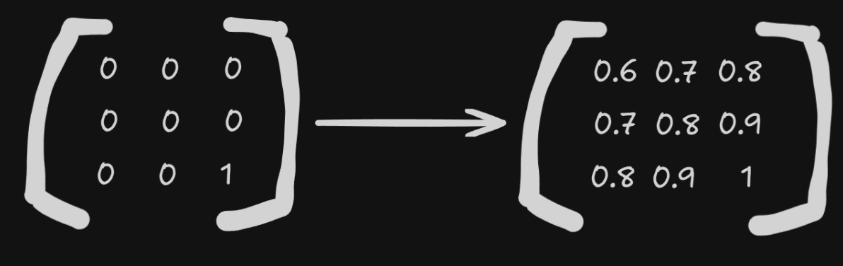
Then we can simply put it in a table mapping each state to it's value - this is called a V-table and has one dimension.
To take an action, our policy simply looks at "which of the states, that are reachable from here, have the highest value according to my table?".
This means that by having the optimal value-function, we also automatically have the optimal policy.
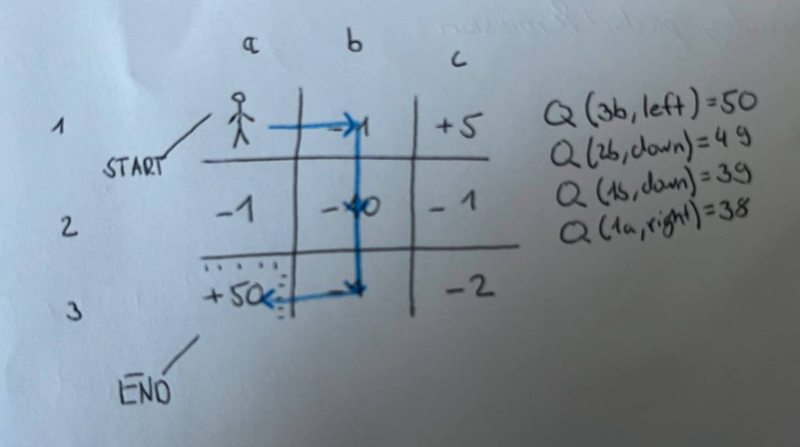
Instead of just the state, we can also map a state-action pair to a value - this is called a Q-table and has two dimensions.
To take an action here, the question becomes: "from the state-action pairs that the same state as my current, which has the highest value?".
The action from this pair, is the one that is taken.
(We will learn later, when the Q-table is more useful.)
This is called model-based learning, where instead we can perfectly simulate the environment mathematically without any unknowns (dynamic programming).
But what is there to learn if we can calculate everything mathematically?
Well, the answer is generalization.
We can do this by putting the agent in multiple environments and training him partly on each.
After this he should be able to generalize and be ready for an environment we can't / don't model.
So what if we can't actually calculate the value because we don't know beforehand what will happen in this environment.
Then we need to take the experiential and iterative approach during our model-free learning.
One of these is called Monte Carlo (MC).
We first let our agent go through an entire episode.
An episode is a unit of a complete walkthrough of the environment consisting of many steps - one game of pong f.e. would be an episode. It is finished once we reach a terminal state (like reaching the goal or dying) or can be ended with other conditions (like after 50 steps).
At the end we then can sum up all the rewards our agent got throughout it and get the total reward G.
We also know which states our agent has been in - that way we can calculate the value for each of those and construct equations for our value-function.
We then can use this to update our table.
Since we want to generalize, we don't simply replace those values- we iteratively change it over many episodes.
We can do that by letting out agent roam around randomly for X episodes and then taking the average for each value-prediction.
Or let our agent try his luck and update the table each time by multiplying it with a learning rate $\alpha$ (a value between 0 and 1) and adding it to our existing value multiplied by (1 - $a$).
It would then look like this: TODO
The other technique is called Temporal Difference Training (TD).
Instead of having to finish an entire episode before learning (which is why some may refer to this as "unsupervised"), it can do it on a step-by-step basis.
Some environments simply require it: those with very long or endless episodes like trading.
But how can we update the value predictions if we don't know the value?
By training on its own prediction - this is called bootstrapping.
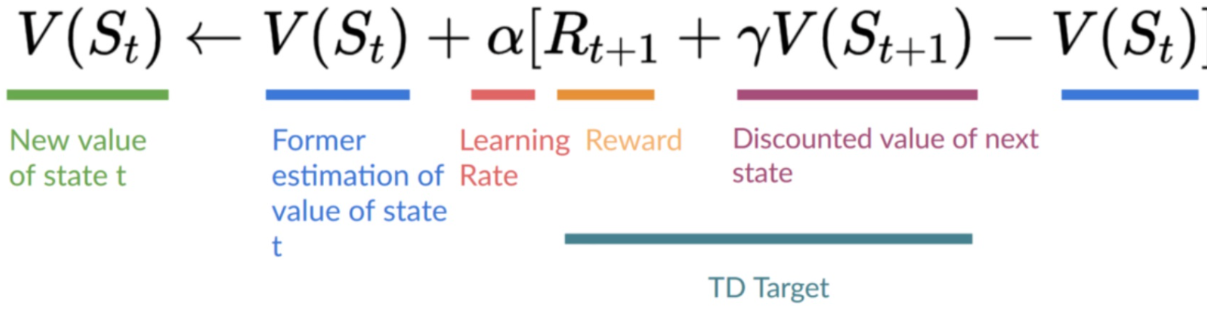
When we take an action to get to a next step, we train the predicted value of the current step $V(S_t)$ by first getting a) the predicted value of the next state $V(S_{t+1})$ b) the immediate reward of the next state take $R_{t+1}$
Using this information we can update the expected value of our current step by applying a discount $\gamma$ to the predicted value of the next step to account for the fact, that it is simply approximating reality and at the beginning of our training run not of use.
So in order to adjust our estimation and train our function, we can do this:
This sound wrong, doesn't it?
Why should we include "corrupt" data, even if accounted for?
Because after a while the results actually "normalize" and we can start to trust the predicted value.
By the way, this is only one of the forms of TD - one where $n=1$, because we trained the state 1 step back.
Bringing $n$ towards $\infty$ (or at least as high as the maximum steps per episode), we see that TD becomes the same as MC - this is because when we can collect all the rewards of an episode we again get the total cumulative reward $G_t$
Increasing $n$, allows us to have a lower bias, because we rely on more actual rewards than predictions.
Interestingly, this also increases variance.
Variance here means how much the value of a state varies from episode to episode.
Having been in a state, our agent could go into one which has a strong reward.
Even though this only happens many steps into the future, in MC or high $n$ TD it greatly impacts the calculated value.
Since TD "looks" only few steps into the future it therefore is more stable against random and unexpected rewards.
We can call the data from MC a "noisy observation of the average", which should generalize after throwing some data at it.
However, there is still a problem with that.
Unfortunately not all environments are simple and without randomness.
Short detour into transition-probabilities.
As an example, imagine Dora the Explorer looking on which path to go to.
We are currently at State $S0$ and have three paths to choose from (so 3 possible actions).
One of the paths leads to an old bridge.
Going over it, there is a 80% chance we get to the other site, and an 20% chance we will fall down and die painfully.
This means that there will be 4 adjacent states, not 3: $[S_1, S_2, S_{3a}, S_{3b}]$.
Like we learned, we can argmax our V-table to get the state with the highest predicted value.
This might return $S_{3a}$, because Dora actually wants to die (because of her fucked up reward-function) and so she sees the value of that state.
However, even if we take the action (going over the bridge), there is still a chance, that we will cross it and reach state $S_{3b}$ instead.
If we are using a model-based approach, this mean we know the probabilities, and can go with this - the value of the states $S_{3a}$ and $S_{3b}$ will naturally follow the probabilities of the environments model.
When training model-free, however, this information is missing.
Naturally, we want our model to learn these probabilities - how can it make a proper choice without this knowledge.
(The same goes for when the reward of a state is random)
By using a Q-table, we can learn it.
The model predict which value the states $S_{3a}$ and $S_{3b}$ have, just like our V-table would.
However, it will also look at the state before that and train the value of our action that brings us towards these two.
It then will understand, that there is an 80% chance, we will get an actually shitty result.
This is where "short-term" learning exceeds - this information isn't "diluted" in the training data.
Here is another way to put it.
TD learns the underlying model of the environment and thus learns the Markov Reward Process (because it learns the mechanics of a single step).
MC simply tries to reduce the mean error of the predicted value to the actual total reward.
MC fits, while TD models.
This is a tradeoff we have to take in account when deciding which to use based on the environment and training goals.
Increasing $n$ means we get more information for each update, but this also means that the information is noisier.
The larger the episode, the higher of an $n$ we can usually get away with.
How much of a problem noise is, is also dependent on how complex the environment (or to be precise: the model behind it) is.
In general, this also leads to us needing less data, because we can rely on bootstrapping while learning in a more "direct" manner - awesome for when data is scarce or expensive.
There is one thing I have been hiding from you.
All this time, we have assumed, that the environment is Markovian, meaning it follows the Markov Property.
The Markov Property states that, future rewards have to depend on only the current state - and not historical information or any hidden variables.
Imagine a dungeon environment where a state either kills you or reveals a treasure, based on if you have flicked another lever in another spot.
The reason why MC tends to win here, is that you can't learn an unreliable model.
Because MC "looks into the future", it can learn to to flick the lever early, because it expects more value from this action in the long run - even if noisy, at least the information exists (unless our $n$ is high enough).
TD on the other hand, converges on a biased view of a state - it "ignores" the information it doesn't know and ends up learning the average of the possible outcomes of the lever being flicked or not.
The same goes for information that is simply hidden - TD fails to learn the model by the single steps, while MC at least gets the prediction of value somehow right.
As an example - let's say we have a hidden variable that holds the battery of our robot - after this goes to 0, we will simply die.
TD doesn't realize this, as it again looks at the single steps and tries to learn the mechanics of each of them.
MC sees the whole picture - it disvalues (even early) states that lower the battery level, because this data is the noisy observations.
Going back to the dungeon: Why can't we just put the information about the lever being flicked in the state?
Yes, a perfect state representation would fix the issue.
However, oftentimes we can't know beforehand which state to model - not every dungeon has this mechanism.
(Dynamic State Representation is an interesting topic I will soon look at.)
TD is also required for live online updates.
Online learning simply means live-learning before the episode ends.
What we instead can do is offline learning, where we collect a dataset which we can reuse instead of having our agent operate in a simulator (or god forbid real world) each time we wan to train it - simply impractical.
(More on that here)
(hybrid approaches)
Now we are going to tie it all together and actually train something.
Q-learning is an off-policy value-based method that uses TD to train its Q-table.
If this sentence didn't paint a clear as sky picture in your head, reread this article and then google the stuff that is still difficult - multiple sources of information help with learning.
Off-policy here is due to the fact that we encourage exploration by picking actions at random at a probability of $\epsilon$ - we call this an $\epsilon$-greedy policy because it otherwise takes the greedy action of picking the best choice
This is used to balance the exploration-exploitation tradeoff - the question of "how much does my agent exploit state/action he already knows he gets rewarded for vs takes more risk by exploring to find even more rewards?".
It will start at a value of 1, then decrease by 0.0005 each epoch until it reaches 0.05.
Look at this function.
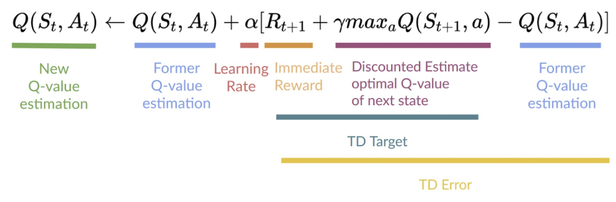
Then compare it to the one I gave you when explaining TD.
That one was called SARSA and is different to Q-learning in one big point.
Let's say we just went from $S_0$ and are now in state $S1$ and the adjacent ones are $[S_2, S_3]$.
Now our function predicts that $S_2$ is the best one.
However, due to the fact that we take random actions, our policy decides that the next state will be $S_3$.
Before we go there however, we still need to update the Q-table for our action we took at $S_0$.
In SARSA, we would train on what the policy actually did - that means that the estimated value of the next state, will be of state $S_3$, which is "grounded in reality".
Q-learning however, instead "assumes", that we will go where the value function tells us to, so $S_2$, even though we aren't going to go there.
As a result it will for example avoid going next to a cliff, because it understands that the random action might just send it to its death.
Q-learning will instead learn to "trust its instincts" and thus take the more efficient path, even though there are cliffs nearby.
Q-learning is a prime example of off-policy training , SARSA of on-policy training.
What's the difference?
In on-policy training, all the decisions the agent takes during training, are the ones he himself predicts using his function.
Here we use it to alter the behavior of the agent, without teaching it the "unrealities" of the policy itself.
☘